Authoring scientific documents with Markdown & Quarto
Abstract
This workshop will show you how to easily create beautiful scientific documents (html, pdf, websites, books…)—complete with formatted text, dynamic code, and figures with Quarto, an open-source tool combining the powers of Jupyter or knitr with Pandoc to turn your text and code blocks into fully dynamic and formatted documents.
Markup and Markdown
Markup languages
Markup languages control the formatting of text documents. They are powerful but complex and the raw text (before it is rendered into its formatted version) is visually cluttered and hard to read.
Examples of markup languages include LaTeX and HTML.
- Tex (often with the macro package LaTeX) is used to create pdf.
\documentclass{article}
\title{My title}
\author{My name}
\usepackage{datetime}
\newdate{date}{24}{11}{2022}
\date{\displaydate{date}}
\begin{document}
 \maketitle
 \section{First section}
 Some text in the first section.
\end{document}
- HTML (often with css or scss files to customize the format) is used to create webpages.
<!DOCTYPE html>
<html lang="en-US">
  <head>
    <meta charset="utf-8" />
    <meta name="viewport" content="width=device-width" />
    <title>My title</title>
    <address class="author">My name</address>
    <input type="date" value="2022-11-24" />
  </head>
  <h1>First section</h1>
  <body>
    Some text in the first section.
  </body>
</html>
Markdown
A number of minimalist markup languages intend to remove all the visual clutter and complexity to create raw texts that are readable prior to rendering. Markdown (note the pun with “markup”), created in 2004, is the most popular of them. Due to its simplicity, it has become quasi-ubiquitous. Many implementations exist which add a varying number of features (as you can imagine, a very simple markup language is also fairly limited).
Markdown files are simply text files and they use the .md extension.
Basic Markdown syntax
In its basic form, Markdown is mostly used to create webpages. Conveniently, raw HTML can be included whenever the limited markdown syntax isn’t sufficient.
Here is an overview of the Markdown syntax supported by many applications.
Pandoc and its extended Markdown syntax
While the basic syntax is good enough for HTML outputs, it is very limited for other formats.
Pandoc is a free and open-source markup format converter. Pandoc supports an extended Markdown syntax with functionality for figures, tables, callout blocks, LaTeX mathematical equations, citations, and YAML metadata blocks. In short, everything needed for the creation of scientific documents.
Such documents remain as readable as basic Markdown documents (thus respecting the Markdown philosophy), but they can now be rendered in sophisticated pdf, books, entire websites, Word documents, etc.
And of course, as such documents remain text files, you can put them under version control with Git.
---
title: My title
author: My name
date: 2022-11-24
---
# First section
Some text in the first section.
Literate programming
Literate programming is a methodology that combines snippets of code and written text. While first introduced in 1984, this approach to the creation of documents has truly exploded in popularity in recent years thanks to the development of new tools such as R Markdown and, later, Jupyter notebooks.
Quarto
How it works
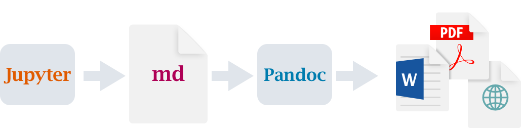
Quarto files are transformed into Pandoc’s extended Markdown by Jupyter (when used with Python or Julia) or by knitr (when used with R), then pandoc turns the Markdown document into the output of your choice.
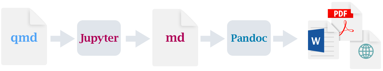
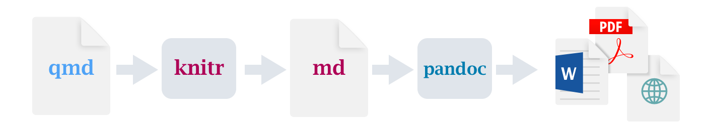
Quarto files use the extension .qmd.
When using R, you can use Quarto directly from RStudio: if you are used to R Markdown, Quarto is the new and better R Markdown.
When using Python or Julia, you can use Quarto directly from a Jupyter notebook (with .ipynb extension).
In this workshop, we will see the most general workflow: simply using a text editor.
Supported languages
Quarto renders highlighting in countless languages and generates dynamic output for code blocks in:
- Python
- R
- Julia
- Observable JS
You can render documents in a wide variety of formats:
Supported outputs (click to expand)
- HTML
- MS Word
- OpenOffice
- ePub
- Revealjs
- PowerPoint
- Beamer
- GitHub Markdown
- CommonMark
- Hugo
- Docusaurus
- Markua
- MediaWiki
- DokuWiki
- ZimWiki
- Jira Wiki
- XWiki
- JATS
- Jupyter
- ConTeXt
- RTF
- reST
- AsciiDoc
- Org-Mode
- Muse
- GNU
- Groff
Installation
-
Download Quarto here.
-
Download the language(s) (R, Python, or Julia) you will want to use with Quarto as well as their corresponding engine (knitr for R; Jupyter for Python and Julia):
If you want to use Quarto with R, you will need:
- R (download here if you don’t have R already on your system),
- the
rmarkdownpackage. For this, launch R and run:
install.packages("rmarkdown")
If you want to use it with Python, you will need:
- Python 3 (download here if don’t have it on your system),
- JupyterLab. For this, open a terminal and run:
python3 -m pip install jupyterlab  # if you are on MacOS or Linux
py -m pip install jupyterlab       # if you are on Windows
Finally, if you want to use Quarto with Julia, you will need:
- Julia (download here if you don’t have Julia),
- the IJulia and Revise packages. For this, launch Julia and run:
] add IJulia Revise
# <Backspace>
using IJulia
notebook()      # to install a minimal Python+Jupyter distribution
Running notebook() allows you to install Jupyter if you don’t already have it.
Document structure and syntax
Front matter
Written in YAML. Sets the options for the document. Let’s see a few examples.
---
title: "My title"
author: "My name"
format: html
---
---
title: "My title"
author: "My name"
format:
  html:
    toc: true
    css: <my_file>.css
---
The above examples would work if you don’t use any code blocks or if you use R code blocks. If you use Python or Julia however, you need to add a jupyter entry with the name of the language that should run in Jupyter.
---
title: "My title"
author: "My name"
format: docx
jupyter: python3
---
---
title: "Some title"
subtitle: "Some subtitle"
institute: "Simon Fraser University"
date: "2022-11-24"
execute:
  error: true
  echo: true
format:
  revealjs:
    theme: [default, custom.scss]
    highlight-style: monokai
    code-line-numbers: false
    embed-resources: true
jupyter: julia-1.8
---
See the Quarto documentation for an exhaustive list of options for all formats.
Written sections
Written sections are written in Pandoc’s extended Markdown.
Code blocks
If all you want is syntax highlighting of the code blocks, use this syntax:
```{.language}
<some code>
```
If you want syntax highlighting of the blocks and for the code to run, use instead:
```{language}
<some code>
```
In addition, options can be added to individual code blocks:
```{language}
#| <some option>: <some option value>

<some code>
```
Rendering
Using Quarto is very simple: there are only two commands you need to know.
In a terminal, simply run either of:
quarto render <file>.qmd     # this will render the document
quarto preview <file>.qmd    # this will display live preview as you work on your document
Let’s give this a try
Create a file called test.qmd with the text editor of your choice.
nano test.qmd
Add a minimal front matter with the output format.
---
title: "Some title"
format: revealjs
---
Then open a new terminal, cd to the location of the file, and run the command:
quarto preview test.qmd
This will open the rendered document in your browser.
We will play with this test.qmd file and see how it is rendered by Quarto as we go.
Examples
Below are a few basic example files and their outputs.
Revealjs presentation
Code
---
title: "My title"
author: "My name"
institute: "Simon Fraser University"
format:
revealjs:
highlight-style: monokai
code-line-numbers: false
embed-resources: true
---
## First section
When exporting to revealjs, second level sections mark the start of new slides,
with a slide title.
This can be changed in options.
---
New slides can be started without titles this way.
# There are title slides
## Formatting
Text can be rendered *in italic* or **in bold** as well as [underlined]{.underline}.
You can use superscripts^2^, subscripts~test~, ~~strikethrough~~, and `inline code`.
> This is a quote.
## Columns
:::: {.columns}
::: {.column width="30%"}
You can create columns.
:::
::: {.column width="70%"}
And you can set their respective width.
:::
::::
## Lists
::: {.incremental}
- List can happen one line at a time
- like
- this
:::
## Lists
- Or all at the same time
- like
- that
## Ordered lists
1. Item 1
2. Item 2
3. Item 3
## Images

## Tables
| Col 1 | Col 2 | Col 3 |
|------ |-------|--------|
| a | 1 | red |
| b | 2 | orange |
| c | 3 | yellow |
:::{.callout-note}
Tables can be fully customized (or you could use raw html).
:::
## Equations
$$
\frac{\partial \mathrm C}{ \partial \mathrm t } + \frac{1}{2}\sigma^{2} \mathrm S^{2}
\frac{\partial^{2} \mathrm C}{\partial \mathrm C^2}
+ \mathrm r \mathrm S \frac{\partial \mathrm C}{\partial \mathrm S}\ =
\mathrm r \mathrm C
$$
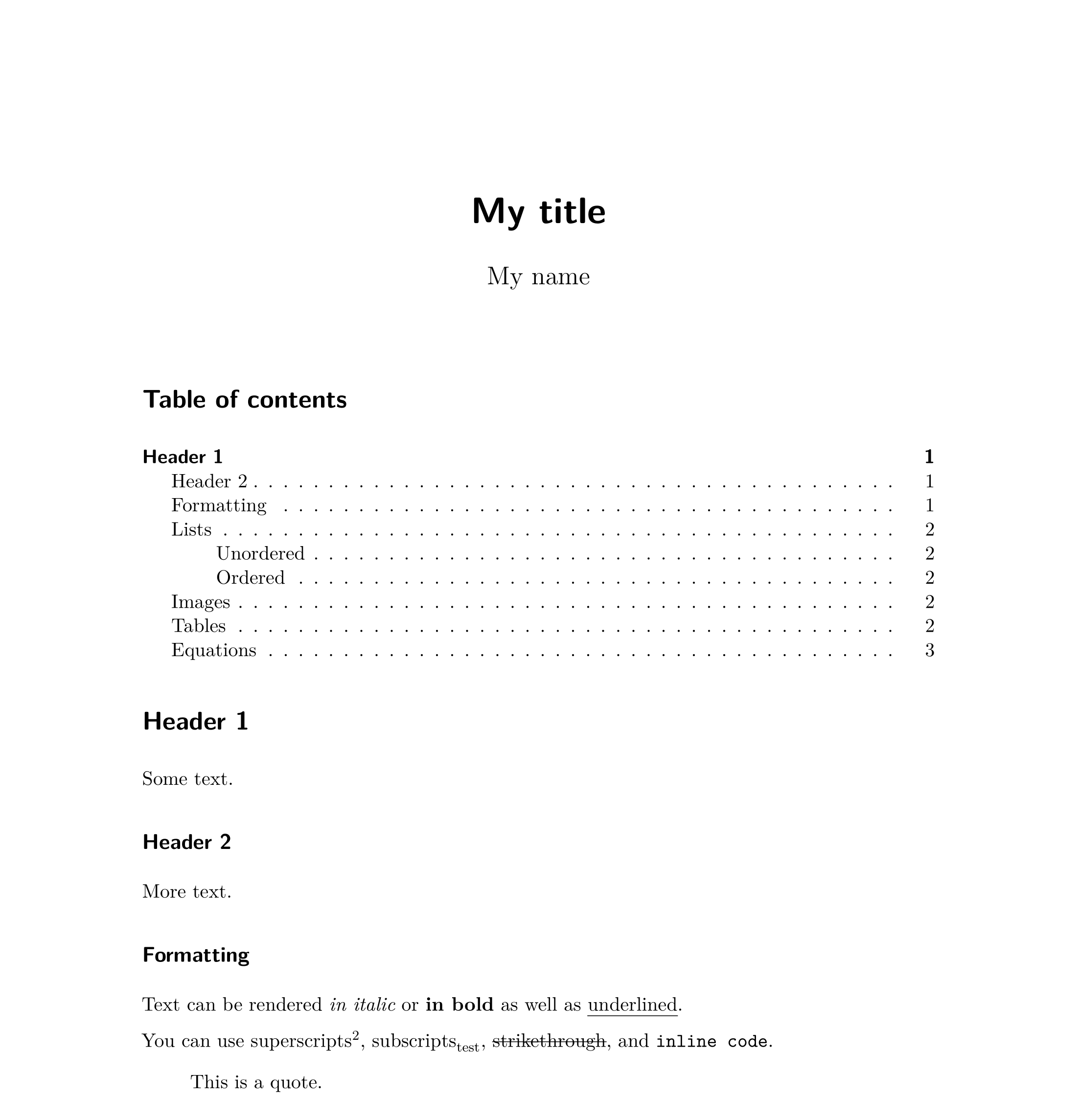
Rendered document

Code
---
title: "My title"
author: "My name"
format:
pdf:
toc: true
---
# Header 1
Some text.
## Header 2
More text.
## Formatting
Text can be rendered *in italic* or **in bold** as well as [underlined]{.underline}.
You can use superscripts^2^, subscripts~test~, ~~strikethrough~~, and `inline code`.
> This is a quote.
## Lists
### Unordered
- Item 1
- Item 2
- Item 3
### Ordered
1. Item 1
2. Item 2
3. Item 3
## Images

## Tables
| Col 1 | Col 2 | Col 3 |
|------ |-------|--------|
| a | 1 | red |
| b | 2 | orange |
| c | 3 | yellow |
:::{.callout-note}
Tables can be fully customized (or you could use raw html).
:::
## Equations
$$
\frac{\partial \mathrm C}{ \partial \mathrm t } + \frac{1}{2}\sigma^{2} \mathrm S^{2}
\frac{\partial^{2} \mathrm C}{\partial \mathrm C^2}
+ \mathrm r \mathrm S \frac{\partial \mathrm C}{\partial \mathrm S}\ =
\mathrm r \mathrm C
$$
Rendered document
quarto install tool tinytex
HTML with R code blocks
Code
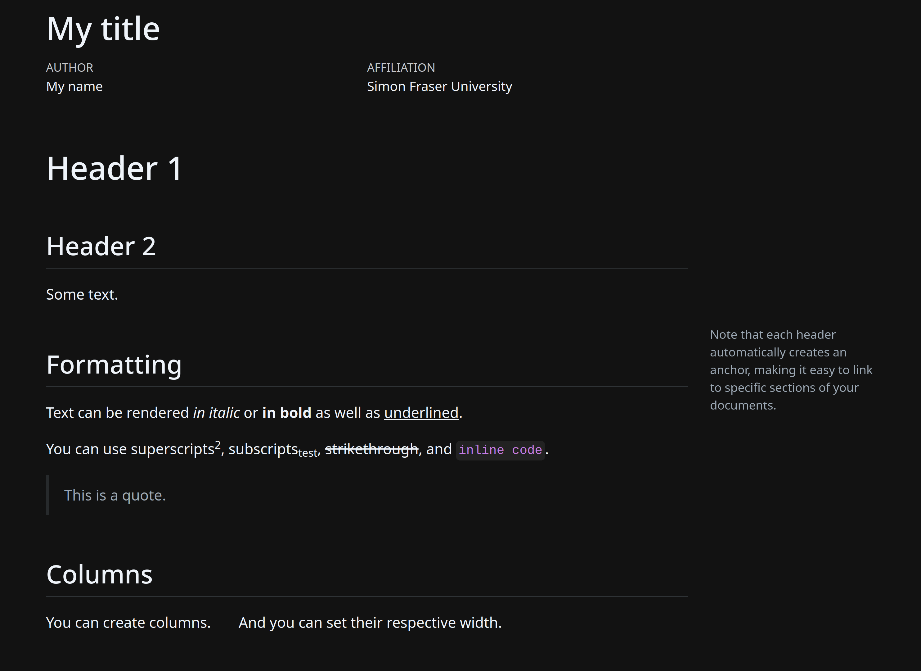
---
title: "My title"
author: "My name"
institute: "Simon Fraser University"
format: html
---
# Header 1
## Header 2
Some text.
## Formatting {#sec-formatting}
::: aside
Note that each header automatically creates an anchor,
making it easy to link to specific sections of your documents.
:::
Text can be rendered *in italic* or **in bold** as well as [underlined]{.underline}.
You can use superscripts^2^, subscripts~test~, ~~strikethrough~~, and `inline code`.
> This is a quote.
## Columns
:::: {.columns}
::: {.column width="30%"}
You can create columns.
:::
::: {.column width="70%"}
And you can set their respective width.
:::
::::
## Lists
- Item 1
- Item 2
- Item 3
## Ordered lists
1. Item 1
2. Item 2
3. Item 3
## Images

## Tables
| Col 1 | Col 2 | Col 3 |
|------ |-------|--------|
| a | 1 | red |
| b | 2 | orange |
| c | 3 | yellow |
:::{.callout-note}
Tables can be fully customized (or you could use raw html).
:::
## Equations
$$
\frac{\partial \mathrm C}{ \partial \mathrm t } + \frac{1}{2}\sigma^{2} \mathrm S^{2}
\frac{\partial^{2} \mathrm C}{\partial \mathrm C^2}
+ \mathrm r \mathrm S \frac{\partial \mathrm C}{\partial \mathrm S}\ =
\mathrm r \mathrm C
$$
## Cross-references
See @sec-formatting.
*Note that you can add bibliographies, flow charts, the equivalent of HTML "div",
and just so much more. Remember that this is a tiny overview.*
## Let's try some code blocks now
```{r}
# This is a block that runs
2 + 3
```
::: aside
Did you notice that the content of your code blocks can be copied with a click?
Of course, this is customizable.
:::
```{.r}
# This is a block that doesn't run
2 + 3
```
```{r}
#| echo: false
# And this is a block showing only the output
data.frame(
country = c("Canada", "USA", "Mexico"),
var = c(2.9, 3.1, 4.5)
)
```
## Plots
```{r}
plot(cars)
```
<br>
You can play with options to add a title:
```{r}
#| fig-cap: "Stopping distance as a function of speed in cars"
plot(cars)
```
<br>
You can have more complex multi-plot layouts:
```{r}
#| layout-ncol: 2
#| fig-cap:
#| - "Stopping distance as a function of speed in cars"
#| - "Vapor pressure of mercury as a function of temperature"
plot(cars)
plot(pressure)
```
For those who have `ggplot2`[^1], you can try that too:
```{r}
library(ggplot2)
ggplot(data = mpg, mapping = aes(x = displ, y = hwy)) +
geom_point(mapping = aes(color = class)) +
geom_smooth()
```
[^1]: You can install it with:
```{.r}
install.packages("ggplot2")
```
Rendered document
Beamer with Python code blocks
Beamer is LaTeX presentation framework: a way to create beautiful pdf slides.
Code
---
title: "Some title"
author: "Some name"
format: beamer
jupyter: python3
---
## First slide
With some content
## Formatting
Text can be rendered *in italic* or **in bold** as well as [underlined]{.underline}.
You can use superscripts^2^, subscripts~test~, ~~strikethrough~~, and `inline code`.
## Lists
- Item 1
- Item 2
- Item 3
## Ordered lists
1. Item 1
2. Item 2
3. Item 3
## Images

## Tables
| Col 1 | Col 2 | Col 3 |
|------ |-------|--------|
| a | 1 | red |
| b | 2 | orange |
| c | 3 | yellow |
:::{.callout-note}
Tables can be fully customized (or you could use raw html).
:::
## Equations
$$
\frac{\partial \mathrm C}{ \partial \mathrm t } + \frac{1}{2}\sigma^{2} \mathrm S^{2}
\frac{\partial^{2} \mathrm C}{\partial \mathrm C^2}
+ \mathrm r \mathrm S \frac{\partial \mathrm C}{\partial \mathrm S}\ =
\mathrm r \mathrm C
$$
## Some basic code block
```{python}
#| echo: true
2 + 3
```
## Some plot
```{python}
import matplotlib.pyplot as plt
import numpy as np
# Data for plotting
t = np.arange(0.0, 2.0, 0.01)
s = 1 + np.sin(2 * np.pi * t)
fig, ax = plt.subplots()
ax.plot(t, s)
ax.set(xlabel='time (s)', ylabel='voltage (mV)',
title='Here goes the title')
ax.grid()
fig.savefig("test.png")
plt.show()
```
Rendered document